Welcome to part 1 to a series of posts regarding my college tuition project!

In this project, I predict the tuition of colleges around the US using data from the National Center for Education Statistics. I chose features I thought would best predict college tuition, such as admission rate, graduation rate, and college location, and I ended up with roughly 20 features.
Data Visualization
Always the first process you should do with your data is to visualize it. Here, I created various plots of tuition vs. various factors I thought would be the best predictors using Seaborn.
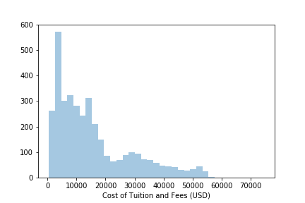
Histogram of Tuition
From this graph, I can tell that tuition is right skewed with peak of around 8000$.
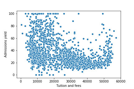
Scatterplot of Tuition and Admissions Rate
While admissions rate seems much more varied from 0-20000$, the rate appears to generally decrease.
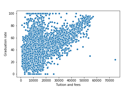
Scatterplot of Tuition and Graduation Rate
Again, a similar trend where graduation rate varies a lot from 0-20000$ but exhibits an increase afterwards.
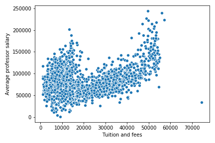
Scatterplot of Tuition and Professor Salary
As expected, as tuition increases, professors' salaries also increases. From these graphs, I predict that my models will be able to predict college tuition more accurately around 30,000$ because of its lower variability in factors like graduation rate.
Data Preparation
The data.csv file contains the colleges as rows and features (including tuition) as columns. I will be using Pandas for loading data and scikit-learn for preprocessing.
import pandas as pd
import joblib

import sklearn.preprocessing as preprocessing
from sklearn.model_selection import train_test_split
from sklearn.compose import ColumnTransformer
from sklearn.pipeline import Pipeline
from sklearn.impute import SimpleImputer
I removed the colleges that didn't have tuition filled in, as well as the rows which have less than 18 out of the 25 features so that there are enough features to predict tuition. This left about 2900 colleges from the original total of 7000.
data = pd.read_csv('data/data.csv')
data = data[pd.notnull(data['Tuition and fees'])]

min_fields = 18
for index, row in data.iterrows():
    filled = 0

    for name, field in row.items():
        if str(field) != 'nan':
            filled += 1

    if filled <= min_fields:
        data.drop(index, inplace=True)
        data.drop(data.columns[[0, 1, 2]], axis=1, inplace=True)
Split data into train and test sets using train_test_split() with 80% of the data going into the train set.
data = data.reset_index(drop=True)
train, test = train_test_split(data, test_size=0.2)
X_train, y_train = train.drop(train.columns[[2]], axis=1), train.iloc[:,2]
X_test, y_test = test.drop(test.columns[[2]], axis=1), test.iloc[:, 2]
Scale targets between 0 and 1 for faster convergence. While the sklearn libary contains a plethora of scalers, I chose min max scaler because of its simplicity and skewed dataset. I saved the scaler using joblib so I could later scale the predicted targets back.
scaler = preprocessing.MinMaxScaler()
scaler.fit(y_train.values.reshape(-1, 1))
y_train, y_test = scaler.transform(y_train.values.reshape(-1, 1)), scaler.transform(y_test.values.reshape(-1, 1))
joblib.dump(scaler, 'min_max_scaler.pkl')
To encode the numeric features, I defined the columns which had numeric features and a Pipeline from sklearn. I first imputed the data (meaning I replaced missing values with the mean) and then scaled the data. For the categorical features, I instead used a OneHotEncoder in a Pipeline to convert the categories to numeric values.
numeric_features = X_train.columns[[0, 1] + [i for i in range(4, 24)]]
numeric_trans = Pipeline(steps=[('imputer', SimpleImputer(strategy='mean')),
('scaler', preprocessing.MinMaxScaler())])

column_features = X_train.columns[[2, 3]]
column_trans = Pipeline(steps=[('encoder', preprocessing.OneHotEncoder(drop='first'))])
I then created a ColumnTransformer by passing the pipelines and feature names and then transformed the data.
transformer = ColumnTransformer(transformers=[('numeric', numeric_trans, numeric_features),
('categorical', column_trans, column_features)],
remainder='passthrough')
transformer.fit(X_train)

X_train = pd.DataFrame(transformer.transform(X_train))
X_test = pd.DataFrame(transformer.transform(X_test))
Now that the data is ready, it's finally time for creating the model in Part 2!
Full code is located over on my GitHub.