Using Matplotlib, a python plotting library, I figured out how to graph both 2d and 3d vector fields along with their associated flow lines. Intuitively, flow lines are curves which you get by starting at a point and tracing in the direction of the vector field. This is the path a particle would take in a vector field.
The formal definition of a flow line is this: Let \(\bf{F}\) be a vector field and \(\bf{x(t)}\) be the flow line. Then \(\bf{x'(t) = F(x(t))}\). In other words, at every point on the path \(\bf{x}\), \(\bf{x}\) is tangent to the vector field \(\bf{F}\).

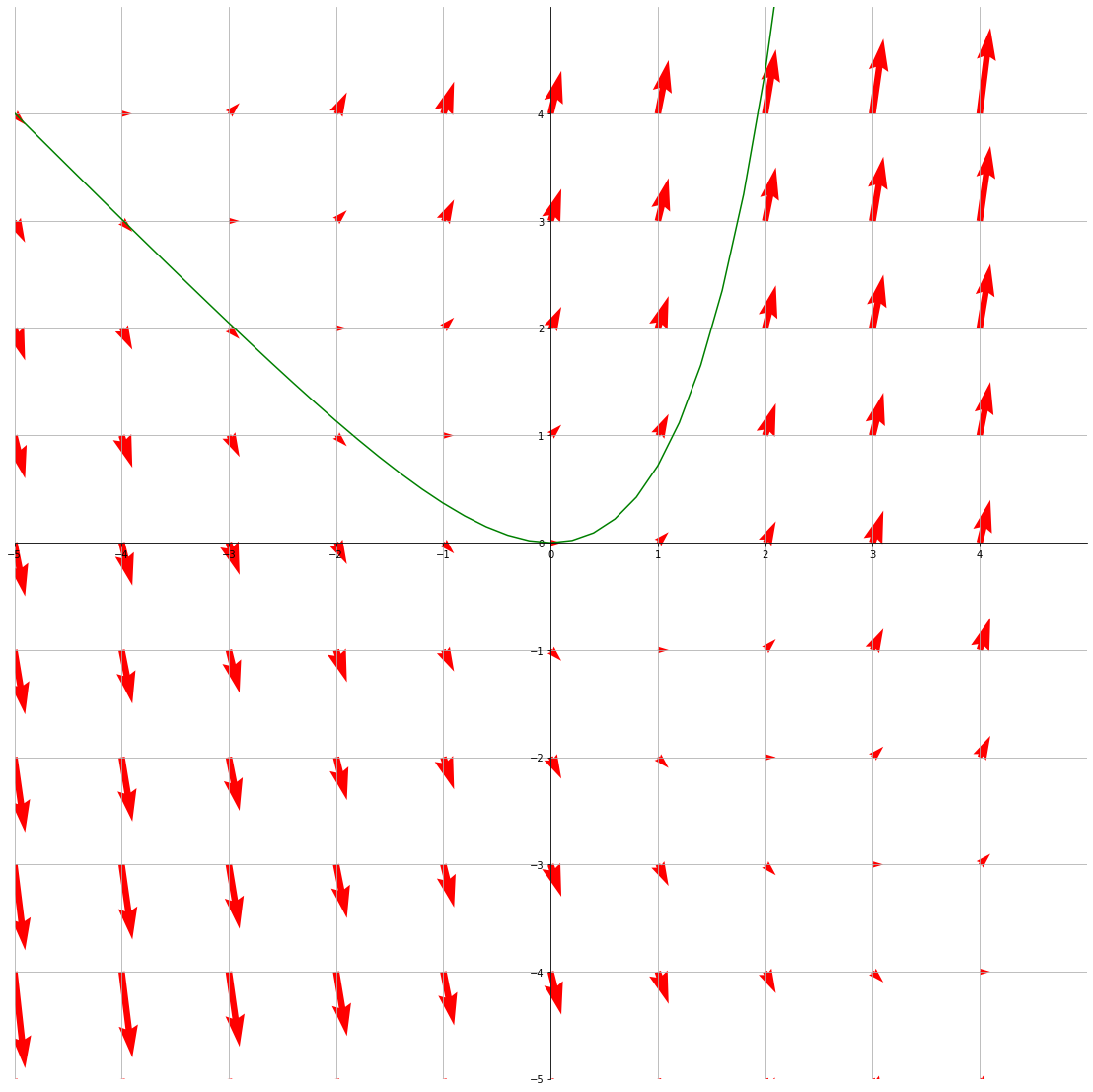
The vector field \(\textbf{F}(x)=(1, x+y)\) with a flow line (green) through the point (0,0)
Graphing in 2d
Graphing a simple vector field
First, we must import all of our dependencies, which are matplotlib and numpy.
import matplotlib.pyplot as plt
import numpy as np
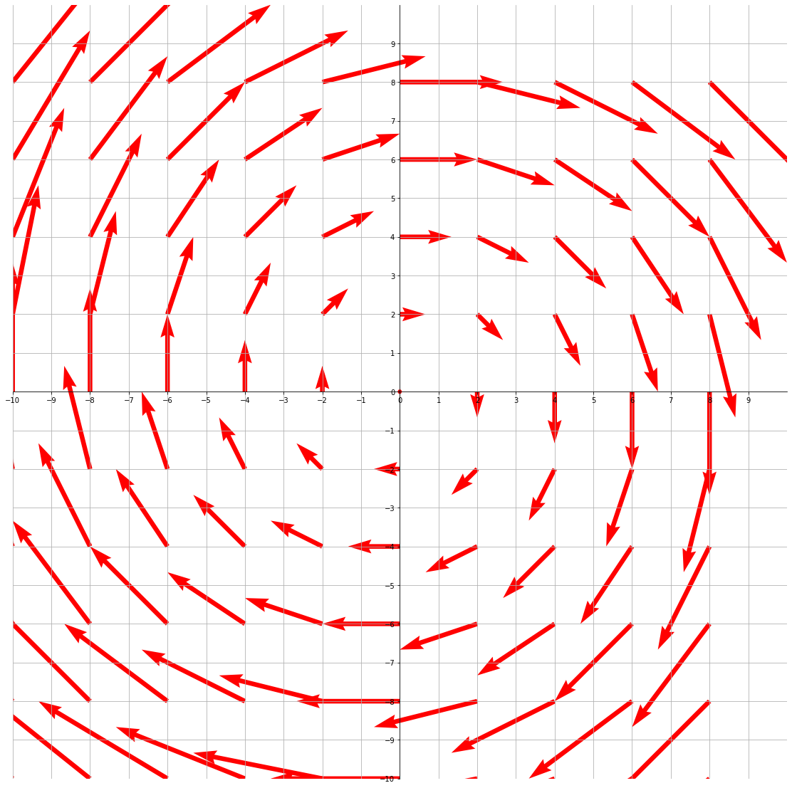
Now we have to define the x and y components of our vector field as a function of the point (x,y). In this case, \(\textbf{F}(x, y) = (y, -x)\). We also define the x and y bounds as well as our step size (which defines our 'grid' of vectors) and scale (which scales the vectors in the graph).
vf_x = lambda x, y: y
vf_y = lambda x, y: -x

x_lim = (-10, 10)
y_lim = (-10, 10)

step = 2
scale = 3
We create a grid using np.meshgrid, where each point in the grid is given by (X[i, j], Y[i, j]), where i and j are indices. We then assign the x component of every vector in the grid to U and the y component to V using our vector field function defined earlier. Matplotlib's quiver function creates the vector field.
X, Y = np.meshgrid(np.arange(x_lim[0], x_lim[1], step), np.arange(y_lim[0], y_lim[1], step))
U = np.zeros(X.shape)
V = np.zeros(Y.shape)

for i in range(X.shape[0]):
    for j in range(Y.shape[0]):
          U[i,j] = vf_x(X[i, j], Y[i, j])
          V[i,j] = vf_y(X[i, j], Y[i, j])

fig, ax = plt.subplots(figsize=(20, 20))
_ = ax.quiver(X, Y, U, V, units='xy', scale=scale, color='red')

plt.xlim(x_lim)
plt.ylim(y_lim)
Finally, we can plot the vector field and make it look at bit nicer.
ax.set_xticks(np.arange(x_lim[0], x_lim[1], 1))
ax.set_yticks(np.arange(y_lim[0], y_lim[1], 1))
ax.set_aspect('equal')

# Move axis to the middle
ax.spines['left'].set_position('zero')

ax.spines['right'].set_color('none')
ax.yaxis.tick_left()

ax.spines['bottom'].set_position('zero')

ax.spines['top'].set_color('none')
ax.xaxis.tick_bottom()
plt.grid()

plt.show()
plt.close()
Plot the vector field (2d)
This is the final result!

The vector field \(\textbf{F}(x, y) = (y, -x)\) with step=2 and scale=3
Graphing Functions
We can also graph functions using plt.plot, including flow lines. func_x is an array of x values, and func_y is an array of y values.
plt.plot(func_x, func_y, 'g')For example, this plots the flowline through (0, 0) for the vector field \(\textbf{F}(x, y) = (1, x+y)\).
func_x = np.arange(-10, 10, 0.2)
func_y = 1*np.exp(func_x) - func_x - 1
The equation for the flow line is \(y=e^x-x-1\) (not derived)

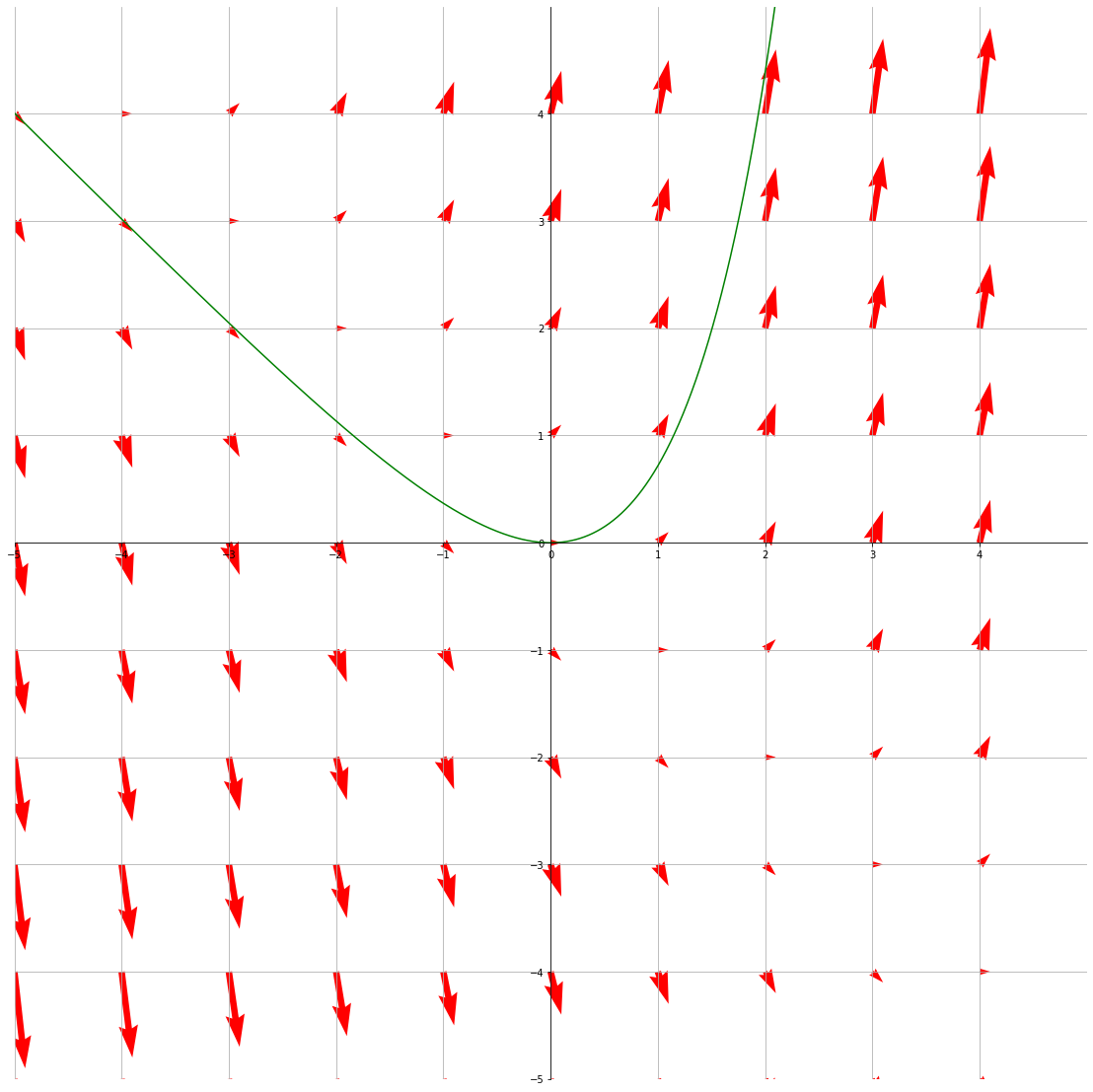
The vector field \(\textbf{F}(x, y) = (1, x+y)\) with a flow line through (0, 0)
Graphing Flow Lines using Euler's Method
What if we can't find the equation to the flow line directly? We can use Euler's method, and the premise behind Euler's method is this:
- Start at point (x, y)
- Find the derivative, or slope, at (x, y). The vector field already gives us the x and y components of the derivative!
- Take a step in the direction of the derivative, and get a new point (x, y)
- Repeat steps 1-3 until either x or y are outside the desired bounds
In python, it looks like this:
def numerically_find_flow_line_2d(starting_point, step, vf_x, vf_y, x_lim, y_lim):
    func_x = []
    func_y = []

    # Find the points to the "right" of the point
    x = starting_point[0]
    y = starting_point[1]
    while True:
        func_x.append(x)
        func_y.append(y)

        delta_x = vf_x(x, y)
        delta_y = vf_y(x, y)

        # Normalize to unit vector and scale by 1/step
        magnitude = np.sqrt(delta_x ** 2 + delta_y ** 2)
        delta_x = delta_x / magnitude * step
        delta_y = delta_y / magnitude * step

        # Get the new point
        x = x + delta_x
        y = y + delta_y

        # Break if either x or y is outside of bounds
        if x > x_lim[1] or x < x_lim[0] or y > y_lim[1] or y < y_lim[0]:
            break

        # Break if it's taking too long for the curve to leave the bounds
        if len(func_x) > 10000:
            break

    # Find the points to the "left" of the point- nearly identical
    x = starting_point[0]
    y = starting_point[1]
    while True:
      Here, we insert at the front because these points occur before the starting point instead of the back
        func_x.insert(0, x)
        func_y.insert(0, y)

        delta_x = vf_x(x, y)
        delta_y = vf_y(x, y)

        magnitude = np.sqrt(delta_x ** 2 + delta_y ** 2)
        delta_x = delta_x / magnitude * step
        delta_y = delta_y / magnitude * step

        # Here, we subtract delta instead of add
        x = x - delta_x
        y = y - delta_y

        if x > 5 or x < -5 or y > 5 or y < -5:
            break
        if len(func_x) > 20000:
            break

    return func_x, func_y
numerically_find_flow_line_2d()
Here's the result—it looks identical to the graph we generated by manually finding the flow line! As long as the step size is sufficiently large, the numerically generated flow line should be close to the actual flow line.

The vector field \(\textbf{F}(x, y) = (1, x+y)\) with a flow line through (0, 0)
Graphing in 3d
Well, can we graph vector fields in 3d? Yes! To graph in 3d, we have to add a special import which we will use to create a 3d axis. Other than that, all we have to do is add an extra variable.
from mpl_toolkits.mplot3d import Axes3D
def make_vf_3d(x_lim, y_lim, z_lim, step, vf_x, vf_y, vf_z, length, func_xs=None, func_ys=None, func_zs=None):
    X, Y, Z = np.meshgrid(np.arange(x_lim[0], x_lim[1], step),
                          np.arange(y_lim[0], y_lim[1], step),
                          np.arange(z_lim[0], z_lim[1], step))
    U = np.zeros(X.shape)
    V = np.zeros(Y.shape)
    W = np.zeros(Z.shape)

    # Assign vector components to the U, V, and W arrays
    for i in range(X.shape[0]):
        for j in range(Y.shape[0]):
                for k in range(Z.shape[0]):
                    U[i, j, k] = vf_x(X[i, j, k], Y[i, j, k], Z[i, j, k])
                    V[i, j, k] = vf_y(X[i, j, k], Y[i, j, k], Z[i, j, k])
                    W[i, j, k] = vf_z(X[i, j, k], Y[i, j, k], Z[i, j, k])

    fig = plt.figure(figsize=(10, 10))
    # 3d projection
    ax = fig.gca(projection='3d')

    # Plot the vector field
    ax.quiver(X, Y, Z, U, V, W, length=length, color='red')
    if func_x is not None:
        plt.plot(func_x, func_y, func_z, 'g')

    ax.set_xlim3d(x_lim)
    ax.set_xlim3d(y_lim)
    ax.set_zlim3d(z_lim)
    plt.grid()

    plt.show()
    plt.close()
make_vf_3d()
We can also use Euler's method in 3d as well. It's the same as the 2d way, but we're adding a z variable.
def numerically_find_flow_line_3d(starting_point, step, vf_x, vf_y, vf_z, x_lim, y_lim, z_lim):
    func_x = []
    func_y = []
    func_z = []

    # Find points to the "right" of the starting point
    x = starting_point[0]
    y = starting_point[1]
    z = starting_point[2]
    while True:
        func_x.append(x)
        func_y.append(y)
        func_z.append(z)

        delta_x = vf_x(x, y, z)
        delta_y = vf_y(x, y, z)
        delta_z = vf_z(x, y, z)

        # Scale the deltas
        magnitude = np.sqrt(delta_x ** 2 + delta_y ** 2 + delta_z ** 2)
        delta_x = delta_x / magnitude * step
        delta_y = delta_y / magnitude * step
        delta_z = delta_z / magnitude * step

        # Find the new point
        x = x + delta_x
        y = y + delta_y
        z = z + delta_z

        # Break if the x, y, or z variable is out of bounds
        if x > x_lim[1] or x < x_lim[0] or \
            y > y_lim[1] or y < y_lim[0] or \
            z > z_lim[1] or z < z_lim[0]:
            break

        # Break if it's taking too long
        if len(func_x) > 50000:
            break

    # Find points to the "left" of the starting point
    x = starting_point[0]
    y = starting_point[1]
    z = starting_point[2]
    while True:
        func_x.insert(0, x)
        func_y.insert(0, y)
        func_z.insert(0, z)

        delta_x = vf_x(x, y, z)
        delta_y = vf_y(x, y, z)
        delta_z = vf_z(x, y, z)

        magnitude = np.sqrt(delta_x ** 2 + delta_y ** 2 + delta_z ** 2)
        delta_x = delta_x / magnitude * step
        delta_y = delta_y / magnitude * step
        delta_z = delta_z / magnitude * step

        x = x - delta_x
        y = y - delta_y
        z = z - delta_z

        if x > x_lim[1] or x < x_lim[0] or \
            y > y_lim[1] or y < y_lim[0] or \
            z > z_lim[1] or z < z_lim[0]:
            break
        if len(func_x) > 100000:
            break

    return func_x, func_y, func_z
numerically_find_flow_line_3d()
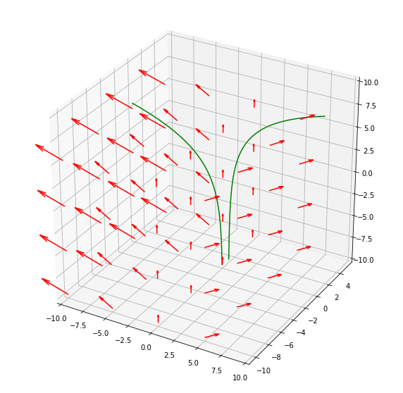
Here is a result:

Graphing the vector field \(F(x, y, z) = (x, 0, 3)\) with two different flow lines starting at (1, 1, 2) and (-3, 0, 2)