Welcome to my first post in a series on deep reinforcement learning in Pytorch. Reinforcement learning is a branch of machine learning dealing with agents and how they make decisions in an environment. RL can be used to play games from snake to Starcraft or even to trade stocks.
OpenAI Gym's Lunar Lander Environment
In this post, I'm going to teach you how to implement deep q learning, a simple deep reinforcement learning algorithm, in Pytorch.
Terminology
The environment is where the agent makes decisions, which is represented by a state vector. The goal of the agent is to maximize total reward.
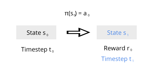
Agent in an environment
At timestep \(t=0\), the environment has a state \(s_0\). The agent then takes an action \(a_0\) according to a policy \(\pi\) (which just tells the agent to take an action from a given state), and receives a reward \(r_0\) and the next state \(s_1\). One way of finding a good policy is using deep Q learning. Each episode consists of all state, actions, and rewards from beginning to end.
The Algorithm
Reinforcement learning using neural networks is unstable and difficult to train. However, deep Q learning introduces several improvements which makes deep reinforcement learning more feasible:
- It uses a replay buffer, which stores the last \(n\) experiences that consist of a state, action, reward, next state, and done tuple. The learning is based by sampling minibatches from the replay buffer, thereby removing the high correlation between experiences.
- It uses off-policy learning. There are 2 Q networks, a local (which is being optimized) and a target (periodically updated by the local network) network. Learning off-policy helps decrease correlation between the local and target expected rewards (explained later).
Q Networks
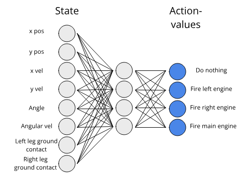
Example Q network for the Lunar Lander environment
In deep Q learning, Q networks are neural networks trained to select the best action. The input to a Q network is the state vector \(s\) and the output is the action vector \(a\). We train the Q network to output the expected return of each action given a state, so that the action with the highest expected return should be selected. The expected return is just the sum \(\sum_{i=0}^{j} P(R_i) \cdot R_i\) where \(R_i = r_t + r_{t+1} + r_{t+2} + \cdots\).
class DQNModel(nn.Module):
    def __init__(self, state_len, action_len):
        super().__init__()

        self.fc1 = nn.Linear(state_len, 64)
        self.fc2 = nn.Linear(64, 64)
        self.fc3 = nn.Linear(64, action_len)

        self.relu = nn.ReLU()

    def forward(self, x):
        # Takes in a state vector with length state_len and outputs an action vector with length action_len
        x = self.relu(self.fc1(x))
        x = self.relu(self.fc2(x))
        x = self.fc3(x)

        return x
This is an example of a simple Q network which inputs the state vector and outputs the expected returns for each of the possible actions.
The Policy
Deep Q learning uses the epsilon greedy policy. A random action is chosen with probability \(\epsilon\) and an action chosen according to the Q network is chosen with probability \(1-\epsilon\). Epsilon is usually decayed towards 0 so that gradually more of the actions are taken according to the Q network.
    def policy(self, state, eps):
        if random.random() < eps:
            # Random action with probability epsilon
            return self.env.action_space.sample()
        else:
            # Act according to local q network by selecting the action with highest expected return
            self.local_qnetwork.eval()
            with torch.no_grad():
              state = torch.FloatTensor(state).cuda().unsqueeze(0)
                out = self.local_qnetwork(state).cpu()
            self.local_qnetwork.train()

            return torch.argmax(out).item()
This is the policy method, which accepts a state and the epsilon and outputs the action.
Training the Q network
The paper introduces replay buffers which simply hold the most recent experience tuples and act as our dataloader. We then train the network on minibatches sampled from the replay buffer.
class ReplayBuffer:
    def __init__(self, queue_len, device):
        self.queue = deque(maxlen=queue_len)
        self.device = device

    def put(self, experience):
        self.queue.append(experience)

    def batch_get(self, batch_size, state_size):
        if batch_size > len(self.queue):
            experiences = [random.sample(self.queue, 1)[0] for _ in range(batch_size)]
        else:
            experiences = random.sample(self.queue, batch_size)

        states, next_states = torch.zeros((batch_size, state_size)), torch.zeros((batch_size, state_size))
        actions, rewards, dones = torch.zeros((batch_size, 1)), torch.zeros((batch_size, 1)), torch.zeros((batch_size, 1))
        for i, experience in enumerate(experiences):
            states[i] = torch.FloatTensor(experience[0])
            actions[i] = experience[1]
            rewards[i] = experience[2]
            next_states[i] = torch.FloatTensor(experience[3])
            dones[i] = experience[4]
        return states.to(self.device), actions.to(self.device), rewards.to(self.device),\
                next_states.to(self.device), dones.to(self.device)
Here is a simply replay buffer class, which holds experience tuples of state, action, reward, next_state, and done values. It returns these values in separate tensors in the batch_get function.
Given a state, the Q network outputs the expected return for each action. So, we'd expect \(Q(s_1) + r_0 = Q(S_0)\). This is something we can optimize for. In the target rewards \(Q(s_1) + \gamma r_0\) we use a discount factor called \(\gamma\). By increasing or lowering \(\gamma\) we can prioritize optimizing the current reward \(r_0\) or future rewards \(Q(s_1)\) more.
self.optimizer = optim.RMSprop(self.local_qnetwork.parameters())
    def qnetwork_step(self):
        # Get the minibatch of experiences
        states, actions, rewards, next_states, dones = self.replay_buffer.batch_get(self.batch_size, self.state_size)

        target_rewards = rewards + self.gamma * torch.max(self.target_qnetwork(next_states), dim=1)[0].unsqueeze(1) * (1 - dones)
        local_rewards = self.local_qnetwork(states).gather(1, actions.long())

        self.optimizer.zero_grad()
        loss = F.mse_loss(local_rewards, target_rewards)
        loss.backward()
        self.optimizer.step()

        return loss.item()
The agent learns using backpropagation.
This also brings us back to the second improvement of deep Q networks. Rather than using the Q network which is being updated to also get the target rewards, we use a target Q network which is periodically updated by the local Q network. This has been shown to improve stability.
   def agent_step(self, state, eps):
        next_state, reward, done = self.env_step(state, eps)
        if len(self.replay_buffer.queue) < self.replay_start_size:
            return next_state, reward, None, done

        # Update the local q network every local_update_frequency steps
        loss = None
        if self.episode_step % self.local_update_frequency == 0:
            loss = self.qnetwork_step()

        # Update the target q network every target_update_frequency steps
        if self.episode_step % self.target_update_frequency == 0:
            self.target_qnetwork.load_state_dict(self.local_qnetwork.state_dict())

        self.episode_step += 1
        return next_state, reward, loss, done

    def env_step(self, state, eps):
        # Choose an action
        action = self.policy(state, eps)
        # Environment step
        next_state, reward, done, _ = self.env.step(action)

        # Store the experience for later use
        self.replay_buffer.put([state, action, reward, next_state, done])
        return next_state, reward, done
This ties up the DQN agent class.
Finally, we need a training loop. Since the agent_step function does most of the heavy lifting, the training loop is fairly small.
def train(agent, eps, num_episodes):
    for episode in range(num_episodes):
        state = agent.reset()

        total_reward = 0
        episode_step = 0
        for i in range(500):
            next_state, reward, loss, done = agent.agent_step(state, eps)

            total_reward += reward

            episode_step += 1
            state = next_state
            if done:
                break

        # Update epsilon
        eps = max(eps * 0.995, 0.01)
The training loop
Results
I trained the Q network on OpenAI's Lunar Lander environment, which has a continuous state space of 8 and a discrete action space of 4. In this environment, the agent is reward for landing softly and at a certain location. Having a reward of 200 is considered solved.
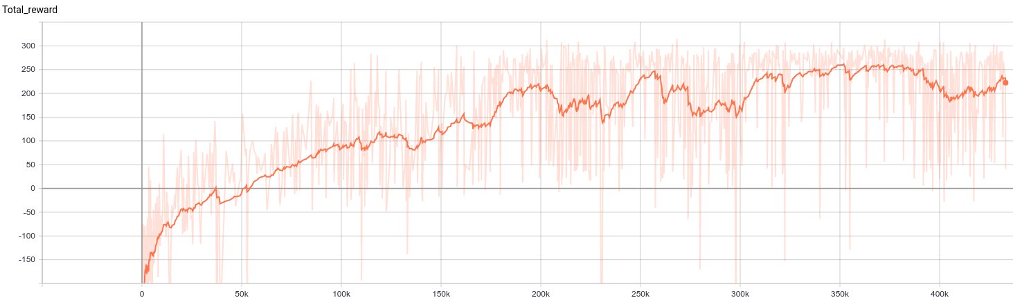
Graph of total rewards vs. steps. The agent appears to average a total reward of 250.
An agent learning how to land a spaceship. As the training progresses, the agent learns how to more efficiently use its fuel.
Improvements
Double DQN
In this paper, the authors introduced a simple improvement to the way the loss is calculated. Instead of calculating target rewards just using the target network, the authors calculated the target rewards by selecting the actions from the local Q network and getting the expected rewards from the target Q network. So the only change we have to make is to change the action selection from the target Q network to the local Q network. This helps remove overestimation of expected rewards.
# How we previously calculated the target_rewards
target_rewards = rewards + self.gamma * torch.max(self.target_qnetwork(next_states), dim=1)[0].unsqueeze(1) * (1 - dones)
# Double DQN
next_target_actions = torch.argmax(self.local_qnetwork(next_states), dim=1).unsqueeze(1)
next_target_rewards = self.target_qnetwork(next_states).gather(1, next_target_actions)
target_rewards = rewards + self.gamma * next_target_rewards * (1 - dones)
Double DQN reward function
Dueling Networks
This paper introduces dueling networks, which alters the Q network behavior. The idea behind dueling networks is instead of just estimating the action-values, it estimates both the state and action values. The agent can now learn which states are valuable regardless of action taken.
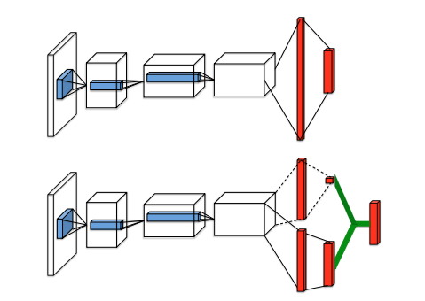
Source: Dueling Network Architectures for Deep Reinforcement Learning
The Q network now consists of shared layers followed by 2 streams which branch off the shared layers. The value stream estimates the expected value of a state, and it's a single number. The advantage stream estimates how much better the actions are relative to each other. Then the final output of the Q network uses both the values from the value and advantage streams, either \(V+A-\text{max} (A)\) or \(V+A- \text{mean}(A)\).
class DQNModel(nn.Module):
    def __init__(self):
        super().__init__()

        self.shared_stream = nn.Sequential(
            nn.Linear(8, 64),
            nn.ReLU()
        )

        self.advantage_stream = nn.Sequential(
            nn.Linear(64, 64),
            nn.ReLU(),
            nn.Linear(64, 4),
        )

        self.value_stream = nn.Sequential(
            nn.Linear(64, 64),
            nn.ReLU(),
            nn.Linear(64, 1)
        )

    def forward(self, x):
        # Takes in a state vector with length 8 and outputs an action vector with length 4
        x = self.shared_stream(state)
        advantages = self.advantage_stream(x)
        value = self.value_stream(x)
        return value + advantages - torch.mean(advantages)
Dueling DQN model
Prioritized Experience Replay
This paper introduces prioritized experience replay. Rather than uniformly sampling from the replay buffer, you prioritize most important experiences. One measure of the importance of experiences is the TD error, which is the absolute value of the difference between target and local rewards. We'd expect that we'd need to learn more from experiences with higher errors. So we can store these TD errors in the experience tuples after we calculate them in the learning step.
td_error = (local_rewards - target_rewards.detach()) ** 2

self.replay_buffer.update_priorities(indices, td_error.data.cpu() + 0.0001)
In the replay buffer class, we calculate the probability of each experience being chosen to be \(\frac{p_i^\alpha}{\sum_{k} p_k^\alpha}\), where \(\alpha\) is a constant designed to control the amount of randomness desired when choosing experiences.
# Get the weights for all experiences
probs = priorities ** self.alpha
probs = probs / np.sum(probs)

# Get the weighted experiences
indices = random.choice(np.arange(len(self.queue)), batch_size, p=probs, replace=False)
experiences = [self.queue[i] for i in indices]
We also have to modify our Q network update step. Because we're sampling from a nonuniform distribution, we have to multiply the TD errors with something called the importance sampling weights, \(w_i = (\frac{1}{N \cdot P(i)})^\beta\). We also can update the priorities for the experiences in the replay buffer. Overall, this makes training faster and more stable.
is_weights = (1 / (len(self.queue) * probs[indices])) ** beta
is_weights /= is_weights.max()

td_error = (local_rewards - target_rewards.detach()) ** 2
loss = torch.mean(is_weights.unsqueeze(1) * td_error)
loss.backward()
The final code is available here.